Unconditional Normalizing Flows for Conditional Generation
Authors: Qiao Sun, Yifan Kang, Eva Zhu
Introduction
Normalizing Flows (NFs) are a long-standing family of modern generative models (Dinh et al., 2015; Rezende & Mohamed, 2015; Kingma et al., 2016). They construct bijective transformations between complex data distributions and simple priors such as Gaussians, enabling exact likelihood computation. Recent advances—such as TARFlow and STARFlow (Zhai et al., 2024; Gu et al., 2024)—significantly improve the fidelity, scalability, and flexibility of flow-based models, reaffirming NFs as a competitive paradigm in generative modeling.
Conditional generation lies at the core of many applications, ranging from class-conditional image synthesis and text-to-image generation to question answering. Unlike unconditional generation, which models a marginal distribution $p(x)$, conditional generation targets the distribution $p(x\mid c)$, where the condition $c$ may be a class label, a text description, or another modality.
A common approach with NFs is to one flow for each condition $c$, or, condition the flow itself. That is, to parameterize a single flow network $f_{\theta}(\cdot\mid c)$ whose behavior explicitly depends on the condition. Conceptually, this means the flow partly learns separate transformations for each condition, rather than a unified representation of the entire dataset.
In this post, we propose an alternative perspective: using a single unconditional Normalizing Flow to model all conditions simultaneously.
Concretely, we train a single flow $f_{\theta}(\cdot)$ on the entire dataset without providing any condition information to the network. This is parameterized by a network with no conditional inputs. To recover the conditional distribution $p(x\mid c)$, we instead assign each condition its own learned prior distribution. These priors adapt during training to capture the distinguishing structure of each condition, while the flow provides a shared, unified latent space.
This design offers several benefits:
- Fast classification.
Besides generation, the model can also be used for classification. Since all data share the same forward transformation, classification can be performed with one flow evaluation, instead of separately forwarding through $f_{\theta}(\cdot\mid c)$ for every possible condition.
- A shared feature space.
The unconditional flow produces a latent representation that tends to cluster inputs with similar semantics. Thus, the learned priors naturally capture condition-specific structure, while the flow acts as a universal feature encoder.
Overall, this unified-flow perspective provides both conceptual simplicity and practical efficiency, revealing that unconditional NFs can naturally support conditional generation—if we shift the modeling burden from the flow to the prior.
Background
Normalizing Flows
Normalizing Flows (NFs) are a class of generative models that establish a bijective transformation between a Gaussian prior distribution $p_0$ and a complex data distribution $p_{\text{data}}$. An NF consists of a forward process and its reverse process. Given a data point $x \in \mathbb{R}^D\sim p_{\text{data}}$, the forward process $\mathcal{F}$ maps it to a prior $z = \mathcal{F}(x)$, where $z$ is trained to follow the Gaussian distribution. The model defines the data likelihood $p(x)$ through the Change of Variables formula. Training proceeds by maximizing the log-likelihood $\log p(x)$ over data samples.
NF requires the forward process $\mathcal{F}$ to be explicitly invertible. Once trained, its exact inverse, $\mathcal{F}^{-1}$, can be used for generation by transforming Gaussian noise back to the data space, i.e. $x=\mathcal{F}^{-1}(z)$ where $z\sim p_0$.
In practice, the forward process is commonly constructed as a composition of multiple simpler bijective transformations $\mathcal{F} := f_{K-1} \circ \cdots \circ f_1\circ f_0$ to enhance its expressiveness. In this way, the log-likelihood objective becomes:
\[\log p(x)=\log p_0(z) + \sum_{i}\log \left|\det\dfrac{\partial f_i(x^i)}{\partial x^i}\right|.\]where $x^0=x$ and $x^{i+1}=f_i(x^{i})$. Here, $\det(\cdot)$ denotes the determinant operator.
More generally, the prior distribution $p_0$ can be any simple distribution with a tractable density, such as a mixture of Gaussians or a pink noise distribution.
Method
In this blog, we investigate a simple setting of class-conditional image generation on the MNIST dataset. Our method is simple: we change the flow network to take no conditional inputs, and assign each class $c$ its own learned Gaussian prior $p(\cdot\mid c) = \mathcal{N}(\mu_c, \sigma_c^2 I)$. Here, $\mu_c$ and $\sigma_c$ are vectors of the same dimension as the input data. This prior is modeled as an pixel-wise independent Gaussian distribution, where each pixel has its own mean and variance.
The training objective becomes:
\[\log p(x\mid c)=\log p_0(z\mid c) + \sum_{i}\log \left|\det\dfrac{\partial f_i(x^i)}{\partial x^i}\right|\] \[=-\frac12\left\|\frac{z-\mu_c}{\sigma_c}\right\|^2 - \sum_t\log \sigma_{c, t} + \sum_{i}\log \left|\det\dfrac{\partial f_i(x^i)}{\partial x^i}\right| + \text{const}\]where the sum over $t$ indexes the dimensions of $z$. Both the flow parameters $\theta$ and the prior parameters ${\mu_c, \sigma_c}$ are learned jointly via maximum likelihood estimation.
At inference time, we only need to sample from the learned Gaussian prior for the desired class, and then invert the flow to generate samples.
Design Choices
We follow the TARFlow architecture (Zhai et al., 2024) as our base flow model and conduct experiments on the MNIST dataset. We use a 6 TARFlow blocks, each with 4 Transformer layers and a hidden size of 256. We use a patch size of 2, resulting in a sequence length of 196 for the 28x28 MNIST images. We use a noise level of 0.1.
Norm Control
To prevent numerical instability and exploding hidden state norms during training, we clip the output of network within a range of $[-3, 3]$.
Initialization of Learned Priors
We parameterize the standard deviation $\sigma_c$ in log-space, i.e. $\log \sigma_c$ as the learned parameter. For simplicity, we initialize $\log \sigma_c$ to zero for all classes, corresponding to an initial standard deviation of 1. However, as specified in later ablations, it turns out that the initialization of $\mu_c$ plays a crucial role in the model’s performance.
Experiments and Ablations
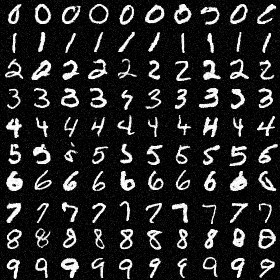
The figure below shows uncrated samples generated by our unconditional flow model with learned priors for each class on MNIST, demonstrating effectiveness of our approach.
Effect of Prior Mean Initialization
We investigate four ways to initialize the prior means $\mu_c$:
- Zero Initialization: All prior means are initialized to zero.
- Random Initialization with Standard Deviation 0.02: Each prior mean is initialized randomly from a standard normal distribution scaled by 0.02. This is a common practice in initializing embedding parameters deep learning.
- Random Initialization with Standard Deviation 1.0: Similar to above, we experiment with a larger scale of 1.0. The generation result above corresponds to this setting.
- Data-based Initialization: Each prior mean is initialized by randomly sampling one data point from the corresponding class (i.e. from 0 to 9 in MNIST).
For each setting, we train the model until convergence and visualize both the generated samples and the learned prior means.
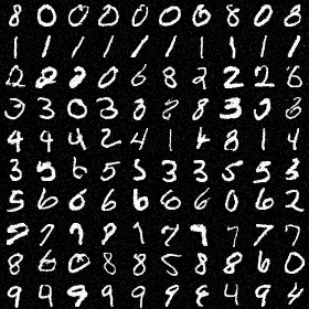
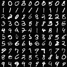

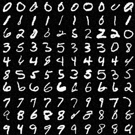
In the generated samples, we observe in setting 1,2,4, there are mixing of similar classes, e.g., 7 and 9, 3 and 5. In contrast, setting 3 with a larger initialization scale of 1.0 produces much cleaner samples with distinct classes.
Our hypothesis is that at initialization, a more ‘separated’ prior space helps the flow learn better class-specific transformations. If the priors are too close together (e.g., all zeros or small random values), the unconditional flow may not see a strong enough signal to differentiate between classes, leading to mode mixing.
The images below show the learned prior means $\mu_c$ for each class under the random initialization and data-based initialization settings.


We can see that the random initialization still learns a somewhat noisy prior mean for each class, while the data-based initialization captures a much clearer structure resembling the actual digits.
We also provide the norm of the $\mu$ over the training process for each setting below:
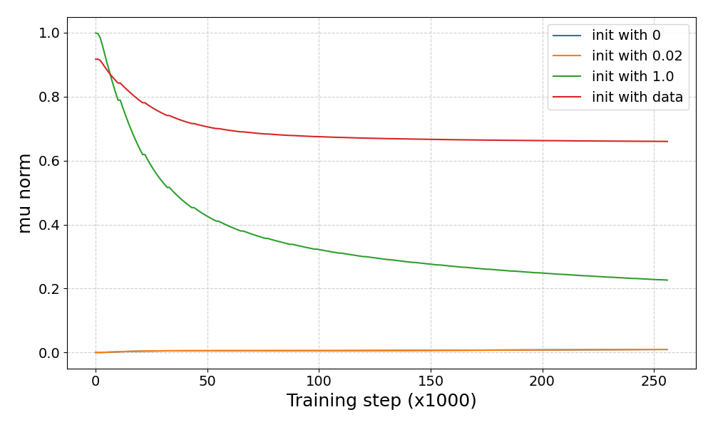
From the plot, one can notice that in all four settings, the norm at convergence basically has the same order of magnitude as at initialization. This suggests that the initial separation of the priors plays a crucial role in guiding the flow to learn distinct class representations.
Conclusion
In this blog post, we explored the idea of using a single unconditional Normalizing Flow with learned class-specific priors for conditional generation. Our experiments on MNIST demonstrate that this simple approach can effectively model class-conditional distributions, provided the prior means are initialized with sufficient separation.
References
- Dinh, Laurent and Krueger, David and Bengio, Yoshua (2015) Nice: Non-linear independent components estimation
- Rezende, Danilo and Mohamed, Shakir (2015) Variational inference with normalizing flows
- Kingma, Diederik P and Salimans, Tim and Jozefowicz, Rafal and Chen, Xi and Sutskever, Ilya and Welling, Max (2016) Improved variational inference with inverse autoregressive flow
- Zhai, Shuangfei and Zhang, Ruixiang and Nakkiran, Preetum and Berthelot, David and Gu, Jiatao and Zheng, Huangjie and Chen, Tianrong and Bautista, Miguel Ángel and Jaitly, Navdeep and Susskind, Joshua M (2024) Normalizing Flows are Capable Generative Models
- Gu, Jiatao and Chen, Tianrong and Berthelot, David and Zheng, Huangjie and Wang, Yuyang and Zhang, Ruixiang and Dinh, Laurent and Bautista, Miguel Angel and Susskind, Josh and Zhai, Shuangfei (2024) STARFlow: Scaling Latent Normalizing Flows for High-resolution Image Synthesis
Enjoy Reading This Article?
Here are some more articles you might like to read next: